
使用 Python Matplotlib 绘制轮廓图
Matplotlib 是 Python 中的免费开源绘图库。它用于使用 Python 脚本创建二维图形和绘图。要使用 matplotlib 功能,我们需要先安装该库。
使用 pip 安装
通过在命令提示符中执行以下命令,我们可以轻松地从 PyPi 安装最新的稳定版 Matplotlib 包。
pip install Matplotlib
您可以通过 conda 安装 Matplotlib,使用以下命令 –
conda install -c conda-forge matplotlib
轮廓图用于通过绘制恒定的 z 切片(称为轮廓)在二维表面可视化三维数据。
它是借助轮廓函数 (Z) 绘制的,该函数是两个输入 X 和 Y(X 轴和 Y 轴坐标)的函数。
Z = fun(x,y)
Matplotlib 提供了两个函数 plt.contour 和 plt.contourf 来绘制轮廓图。
contour() 方法
matplotlib.pyplot. contour() 方法用于绘制轮廓线。它返回 QuadContourSet。以下是此函数的语法 –
contour([X, Y,] Z, [levels], **kwargs)
参数
[X, Y]:可选参数,表示 Z 中的值的坐标。
Z:绘制轮廓的高度值。
levels:用于确定轮廓线/区域的数量和位置。
示例
让我们举一个例子,使用 numpy 三角函数绘制轮廓线。
import numpy as np
import matplotlib.pyplot as plt

def f(x, y):
   return np.sin(x) ** 10 + np.cos(10 + y * x) * np.cos(x)

xlist = np.linspace(-4.0, 4.0, 800)
ylist = np.linspace(-4.0, 4.0, 800)

# 通过这个 numpy 函数创建一个具有给定坐标的网格
X, Y = np.meshgrid(xlist, ylist)
Z = f(X,Y)

fig = plt.figure()
ax = fig.add_axes([0.1, 0.1, 0.8, 0.8])

cp = ax.contour(X, Y, Z)
fig.colorbar(cp) # Add a colorbar to a plot
ax.set_title('Contour Plot')

ax.set_xlabel('x (cm)')
ax.set_ylabel('y (cm)')
plt.show()
输出
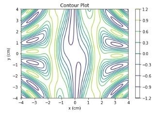
f(x,y) 函数使用 numpy 三角函数定义。
示例
我们再举一个例子,画出轮廓线。
import numpy as np
import matplotlib.pyplot as plt

def f(x, y):
    return np.sqrt(X**2 + Y**2)

xlist = np.linspace(-10, 10, 400)
ylist = np.linspace(-10, 10, 400)

# 创建网格
X, Y = np.meshgrid(xlist, ylist)

Z = f(X, Y)

fig = plt.figure(figsize=(6,5))
ax = fig.add_axes([0.1, 0.1, 0.8, 0.8])

cp = ax.contour(X, Y, Z)
ax.set_title('Contour Plot')
ax.set_xlabel('x (cm)')
ax.set_ylabel('y (cm)')
plt.show()
输出
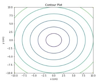
z 函数是 x 和 y 坐标值的平方根之和。使用 numpy.sqrt() 函数实现。
contourf() 函数
matplotlib.pyplot 提供了一种方法 contourf() 来绘制填充轮廓。以下是此函数的语法 –
contourf([X, Y,] Z, [levels], **kwargs)
其中,
[X, Y]:可选参数,表示 Z 中值的坐标。
Z:绘制轮廓的高度值。
levels:用于确定轮廓线/区域的数量和位置。
示例
我们再举一个例子,使用 contourf() 方法绘制轮廓图。
import numpy as np
import matplotlib.pyplot as plt

xlist = np.linspace(-8, 8, 800)
ylist = np.linspace(-8, 8, 800)

X, Y = np.meshgrid(xlist, ylist)
Z = np.sqrt(X**2 + Y**2)

fig = plt.figure(figsize=(6,5))
ax = fig.add_axes([0.1, 0.1, 0.8, 0.8])

cp = ax.contourf(X, Y, Z)
fig.colorbar(cp) # Add a colorbar to a plot
ax.set_title('Filled Contours Plot')
#ax.set_xlabel('x (cm)')
ax.set_ylabel('y (cm)')
plt.show()
输出
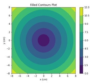
使用 fig.colorbar() 方法,我们为图添加了颜色。z 函数是 x 和 y 坐标值的平方根之和。
示例
在此示例中,我们将使用 matplotlib.plt.contourf() 方法绘制极坐标轮廓图。
import numpy as np
import matplotlib.pyplot as plt

a = np.radians(np.linspace(0, 360, 20))
b = np.arange(0, 70, 10)

Y, X = np.meshgrid(b, a)
values = np.random.random((a.size, b.size))

fig, ax = plt.subplots(subplot_kw=dict(projection='polar'))
ax.set_title('Filled Contours Plot')
ax.contourf(X, Y, values)

plt.show()
输出
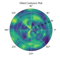
在所有上述示例中,我们都使用了 numpy.meshgrid() 函数来生成 X 和 Y 坐标的数组。
相关文章
有用资源
python 参考教程 - 该教程包含有关 python 的更多信息:https://www.cainiaomax.com/python/