TensorFlow - 制作图表

偏微分方程 (PDE) 是一种微分方程，它涉及具有多个自变量的未知函数的偏导数。 参考偏微分方程，我们将专注于创建新图。

让我们假设有一个尺寸为 500*500 平方的池塘 −

N = 500

现在，我们将计算偏微分方程并使用它形成相应的图形。 考虑下面给出的计算图的步骤。

步骤 1 − 导入库进行仿真。

import tensorflow as tf
import numpy as np
import matplotlib.pyplot as plt

步骤 2 − 包括将二维数组转换为卷积核和简化二维卷积操作的函数。

def make_kernel(a):
   a = np.asarray(a)
   a = a.reshape(list(a.shape) + [1,1])
   return tf.constant(a, dtype=1)

def simple_conv(x, k):
   """A simplified 2D convolution operation"""
   x = tf.expand_dims(tf.expand_dims(x, 0), -1)
   y = tf.nn.depthwise_conv2d(x, k, [1, 1, 1, 1], padding = 'SAME')
   return y[0, :, :, 0]

def laplace(x):
   """Compute the 2D laplacian of an array"""
   laplace_k = make_kernel([[0.5, 1.0, 0.5], [1.0, -6., 1.0], [0.5, 1.0, 0.5]])
   return simple_conv(x, laplace_k)
   
sess = tf.InteractiveSession()

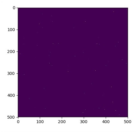
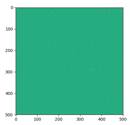
步骤 3 − 包括迭代次数并计算图表以相应地显示记录。

N = 500

# Initial Conditions -- some rain drops hit a pond

# Set everything to zero
u_init = np.zeros([N, N], dtype = np.float32)
ut_init = np.zeros([N, N], dtype = np.float32)

# Some rain drops hit a pond at random points
for n in range(100):
   a,b = np.random.randint(0, N, 2)
   u_init[a,b] = np.random.uniform()

plt.imshow(u_init)
plt.show()

# Parameters:
# eps -- time resolution
# damping -- wave damping
eps = tf.placeholder(tf.float32, shape = ())
damping = tf.placeholder(tf.float32, shape = ())

# Create variables for simulation state
U = tf.Variable(u_init)
Ut = tf.Variable(ut_init)

# Discretized PDE update rules
U_ = U + eps * Ut
Ut_ = Ut + eps * (laplace(U) - damping * Ut)

# Operation to update the state
step = tf.group(U.assign(U_), Ut.assign(Ut_))

# Initialize state to initial conditions
tf.initialize_all_variables().run()

# Run 1000 steps of PDE
for i in range(1000):
   # Step simulation
   step.run({eps: 0.03, damping: 0.04})
   
   # Visualize every 50 steps
   if i % 500 == 0:
      plt.imshow(U.eval())
      plt.show()

图表绘制如下所示 −