Mahotas - 阈值邻接统计
阈值邻接统计 (TAS) 是一种用于从图像中提取任何重要信息的技术。在了解 TAS 的工作原理之前,让我们简要了解一下阈值处理。
阈值处理是一种根据特定值(阈值)将图像分为前景区域和背景区域的技术。前景区域由强度值大于阈值的像素组成。
另一方面,背景区域由强度值小于阈值的像素组成。
TAS 通过计算强度值超过阈值的像素数量来工作。此外,它还考虑了强度值也超过阈值的指定数量的相邻像素。
Mahotas 中的阈值邻接统计
在 Mahotas 中,我们可以使用 mahotas.tas() 和 mahotas.pftas() 函数来计算图像的阈值邻接统计。然后可以使用计算出的统计信息来定位和提取图像中的重要信息。
tas() 函数和 pftas() 函数之间的唯一区别是,在 pftas() 函数中,我们可以设置用于计算 TAS 的任何阈值。
相反,tas() 函数不使用阈值来计算 TAS。
mahotas.tas() 函数
mahotas.tas() 函数将图像作为输入并返回具有阈值邻接统计信息的列表。
语法
以下是 mahotas − 中 tas() 函数的基本语法
mahotas.features.tas(img)
其中,
img −它是输入图像。
示例
在下面提到的示例中,我们使用 mh.tas() 函数计算图像的 TAS 值。
import mahotas as mh
import numpy as np
import matplotlib.pyplot as mtplt
# 加载图像
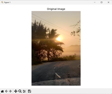
image = mh.imread('sun.png')
# 计算 TAS
tas = mh.features.tas(image)
# 打印 TAS 值
print(tas)
# 为子图创建图形和轴
fig, axis = mtplt.subplots(1, 1)
# 显示原始图像
axes.imshow(image, cmap='gray')
axes.set_title('Original Image')
axes.set_axis_off()
# 调整子图之间的间距
mtplt.tight_layout()
# 显示图形
mtplt.show()
输出
上述代码的输出如下 −
[8.37835351e-01 1.15467657e-02 1.39075269e-02 9.92426122e-03
1.03643093e-02  6.76089647e-03 1.09572672e-02 6.88336269e-03
8.17548510e-03  6.01115411e-02 6.08145111e-03 5.10483489e-03
4.16108390e-03  2.81568522e-03 1.77506830e-03 1.46786490e-03
6.81867008e-04  6.12677053e-04 2.44932441e-04 2.76759821e-04
. . .
4.27349413e-03  7.01932689e-03 4.50541370e-03 5.45604649e-03
6.41356563e-02  4.43892481e-03 4.80936290e-03 4.46979465e-03
3.91413752e-03  2.33898410e-03 3.27299467e-03 1.12872803e-03
2.06353013e-03  4.92334385e-04 1.22371215e-03 1.14772485e-04
6.03149199e-04  3.32444440e-05 3.26112165e-04 1.18730157e-05
1.28228570e-04  0.00000000e+00]
我们得到下面的图像作为输出 −
mahotas.pftas() 函数
mahotas.pftas() 函数将图像和阈值作为输入。它返回具有阈值邻接统计信息的列表。
语法
以下是 mahotas − 中 pftas() 函数的基本语法
mahotas.features.pftas(img, T={mahotas.threshold.otsu(img)})
其中,
img − 是输入图像。
T(可选) −它定义了 TAS 中使用的阈值算法(默认情况下,它使用 Otsu 的方法)。
示例
在下面的例子中,我们使用 mh.pftas() 函数计算图像的 TAS。
import mahotas as mh
import numpy as np
import matplotlib.pyplot as mtplt
# 加载图像
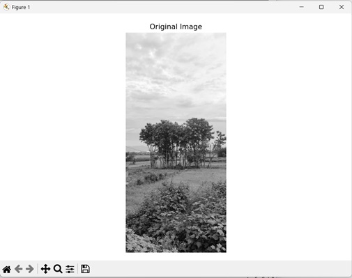
image = mh.imread('nature.jpeg')
# 将其转换为灰度
image = mh.colors.rgb2gray(image).astype(np.uint8)
# 计算无参数 TAS
pftas = mh.features.pftas(image)
# 打印无参数 TAS 值
print(pftas)
# 为子图创建图形和轴
fig, axis = mtplt.subplots(1, 1)
# 显示原始图像
axes.imshow(image, cmap='gray')
axes.set_title('Original Image')
axes.set_axis_off()
# 调整子图之间的间距
mtplt.tight_layout()
# 显示图形
mtplt.show()
输出
以下是上述代码的输出 −
[9.57767091e-01 1.48210628e-02  8.58153775e-03  1.18217967e-02
3.89970314e-03  1.86659948e-03  7.82131473e-04  3.19863291e-04
1.40214046e-04  9.73817262e-01  1.23385295e-02  5.89271152e-03
4.39412383e-03  1.90987201e-03  8.34387151e-04  4.60922081e-04
2.31642892e-04  1.20548852e-04  9.77691695e-01  8.29460231e-03
3.91949031e-03  7.21369229e-03  1.68522833e-03  7.53014919e-04
3.10737802e-04  1.12475646e-04  1.90636688e-05  9.47186804e-01
1.14563743e-02  9.65510102e-03  1.76918166e-02  5.35205921e-03
3.38515157e-03  2.13944340e-03  1.88754119e-03  1.24570817e-03
9.80623501e-01  3.72244140e-03  2.75392589e-03  4.22681210e-03
2.28359248e-03  1.92155953e-03  1.72971300e-03  1.63378974e-03
1.10466466e-03  9.59139669e-01  7.94832237e-03  7.15439233e-03
1.68349257e-02  3.75312384e-03  1.74123294e-03  9.83390623e-04
1.06007705e-03  1.38486661e-03]
得到的图像如下 −
使用平均阈值
我们还可以使用平均阈值计算图像的阈值邻接统计。平均阈值是指通过取图像的平均像素强度值计算出的阈值。
简单来说,阈值是通过将图像中所有像素的强度值相加,然后将该总和除以图像中的总像素数来计算的。
在 mahotas 中,我们首先使用 mean() 函数计算平均阈值。然后,我们在 pftas() 函数的 T 参数中设置此值,以使用平均阈值计算 TAS。
示例
在这里,我们使用平均阈值获取图像的 TAS。
import mahotas as mh
import numpy as np
import matplotlib.pyplot as mtplt
# 加载图像
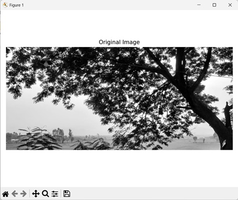
image = mh.imread('tree.tiff')
# 将其转换为灰度
image = mh.colors.rgb2gray(image).astype(np.uint8)
# 计算阈值
threshold = image > np.mean(image)
# 使用平均阈值计算无参数 TAS
pftas = mh.features.pftas(image, Threshold)
# 打印无参数 TAS 值
print(pftas)
# 为子图创建图形和轴
fig, axis = mtplt.subplots(1, 1)
# 显示原始图像
axes.imshow(image, cmap='gray')
axes.set_title('Original Image')
axes.set_axis_off()
# 调整子图之间的间距
mtplt.tight_layout()
# 显示图形
mtplt.show()
输出
执行上述代码后,我们得到以下输出 −
[0.63528106  0.07587514  0.06969174 0.07046435 0.05301355 0.0396411
 0.0278772   0.0187047   0.00945114 0.51355051 0.10530301 0.0960256
 0.08990634  0.06852526  0.05097649 0.03778379 0.02519265 0.01273634
 0.69524747  0.0985423   0.07691423 0.05862548 0.03432296 0.01936853
 0.01058033  0.00482901  0.00156968 0.46277808 0.17663377 0.13243407
 0.10085554  0.06345864  0.03523172 0.01735837 0.00835911 0.00289069
 0.78372479  0.0746143   0.04885744 0.03739208 0.02555628 0.01563048
 0.00822543  0.00436208  0.00163713 0.70661663 0.07079426 0.05897885
 0.06033083  0.04280415  0.02972053 0.01632203 0.01043743 0.00399529]
输出图像如下 −